patchology

Whole slide image (WSI) tiling: tissue detection, artifact removal and square or hexagonal tile grids, on top of OpenSlide or FastSlide.

Many excellent tools already tile WSIs, but most are part of larger frameworks that are heavy to install and hard to navigate when all you need is tiling. patchology is a lightweight, standalone library focused on two things: fast tiling and broad WSI format support.

Warning

For research use only. patchology is not a medical device and is not validated for clinical diagnosis.

Install

Requires Python 3.12+. Both slide backends, OpenSlide and FastSlide, are installed with patchology (OpenSlide's binaries come with openslide-bin, so no system package is needed).

pip install patchology

For development, install from a clone in editable mode, so a git pull takes effect without reinstalling:

git clone https://github.com/twpkevin06222/patchology.git
cd patchology
pip install -e .

Patched OpenSlide (optional)

The standard openslide-bin from PyPI works for most formats. For PreciPoint VMIC (.vmic) support and fixes for Ventana BIF and DICOM, build the patched OpenSlide from the dev branch of twpkevin06222/openslide and install its wheel over the standard one (Linux; needs the build dependencies listed in that repo):

git clone -b dev https://github.com/twpkevin06222/openslide
cd openslide/packaging
./build-wheel.sh
pip install --force-reinstall wheelhouse/openslide_bin-*.whl

Quick start

from patchology import ArtifactConfig, TilingConfig, TilingPipeline, open_slide

pipeline = TilingPipeline(
    tiling=TilingConfig(tile_size=224, tile_mpp=0.5, tile_overlap=0.2, grid="hex"),
    artifacts=ArtifactConfig(pen=True, blur=True),
)
with open_slide("slide.svs", backend="fastslide") as slide:
    result = pipeline.run(slide)
    result.save("out/slide")  # tiles.csv, metadata.json, tissue_mask.png, overlay.png
    for (x, y), tile in result.iter_tiles(slide):
        ...  # tile: (224, 224, 3) uint8 RGB

Or as a generator that owns the slide and exposes its properties and masks:

from patchology import ColorConfig, TileGenerator

with TileGenerator("slide.svs", color=ColorConfig(stain_normalization="macenko")) as gen:
    gen.properties, gen.dimensions, gen.mpp, gen.icc_profile  # no tiling needed
    gen.tissue_mask, gen.artifact_mask, gen.coords, gen.source_stains  # computed in __init__
    for (x, y), tile in gen:  # tissue -> artifacts -> tiles -> ICC (opt-in) -> stain norm
        ...

ROI tiling: pass roi= a GeoJSON file (e.g. a QuPath export, level-0 pixel coordinates) or a folder holding one GeoJSON whose name contains the slide name. Only tissue inside the ROI is tiled. A file whose name does not contain the slide name (whole token, so sample does not match sample-2) is refused unless check_roi_name=False. roi_exclude_classes={"class01"} leaves out objects of those annotation classes (QuPath classification names), e.g. to tile only class02 and class03 from a segmentation annotation file.

with TileGenerator("sample.svs", roi="sample.svs_roi_annotations.geojson") as gen:
    for (x, y), tile in gen:
        ...

Segmentation tiles: SegmentationTileGenerator takes a GeoJSON ground truth and yields ((x, y), tile, mask), with mask a (tile_size, tile_size) uint8 array aligned with the tile. With class_map (annotation class name to label, with integer larger than 0 [default background label value]) each object is drawn with its class's label and objects of unmapped classes are ignored; without it the mask is 0/1. A tile is kept if at least object_mask_overlap (e.g. 0.2 = 20%) of it is ground truth; 0 keeps every tissue tile, including empty masks. All TileGenerator options (ICC, stain normalisation, roi=) apply.

from patchology import SegmentationTileGenerator

with SegmentationTileGenerator(
    "sample.svs",
    "sample.svs_annotations.geojson",
    object_mask_overlap=0.2,
    class_map={"class01": 1, "class02": 2, "class03": 3},
) as gen:
    for (x, y), tile, mask in gen:
        ...

Detection tiles: DetectionTileGenerator takes the same GeoJSON ground truth and yields ((x, y), tile, target), with target = {"boxes": (N, 4) float32, "labels": (N,) int64}: each object's bounding box in COCO [x, y, width, height] tile pixels. An object cut by the tile edge is kept (clipped) if at least min_box_visibility (e.g. 0.6 = 60%) of its box is inside the tile, and a tile is kept if it has at least min_objects objects (0 keeps empty tissue tiles too, as negatives). class_map labels are integers

= 0 (default 1 for every object). With roi_class, unannotated objects outside the annotated region must never count as background: by default tiles lie wholly inside it, and with roi_fill (an RGB colour) tiles only need to overlap it and pixels outside it are painted over, so regions smaller than a tile still give tiles (lower tiling.tissue_overlap for very small regions).

from patchology import DetectionTileGenerator

with DetectionTileGenerator(
    "sample.svs",
    "sample.svs_annotations.geojson",  # ASAP XML: python -m patchology.utilities.xml_to_geojson
    min_box_visibility=0.6,
    min_objects=1,
    class_map={"class01": 1, "class02": 2},
    roi_class="roi",
    roi_fill=(255, 255, 255),  # paint outside the ROI white instead of skipping such tiles
) as gen:
    for (x, y), tile, target in gen:
        ...

GeoJSON format: ROI and ground-truth files are QuPath-style GeoJSON with coordinates in level-0 (full resolution) pixels. See src/patchology/references/sample.svs_annotations.geojson for a complete example. A FeatureCollection (a single Feature, a list of features or a bare geometry also work) of Polygon / MultiPolygon features; the class is read from properties.classification.name, and other geometry types (points, lines) are skipped with a warning:

{
  "type": "FeatureCollection",
  "features": [
    {
      "type": "Feature",
      "geometry": {
        "type": "Polygon",
        "coordinates": [[[22575, 31840], [22575, 31842], "...", [22575, 31840]]]
      },
      "properties": {
        "objectType": "annotation",
        "classification": {"name": "class02", "color": [37, 46, 201]}
      }
    }
  ]
}

The first ring of a polygon is its outline and any further rings are holes.

PyTorch: a generator is a map-style dataset (len, gen[i]), so wrap it in a torch.utils.data.Dataset and use any num_workers; each worker reopens the slide, and tiling runs once in the main process. With the fastslide backend, start workers with multiprocessing_context="forkserver" (or "spawn"): FastSlide's thread pool does not survive fork(), so forked workers raise instead of reading. Read tiles with gen.get_tile(i) (((x, y), tile), plus mask for segmentation), gen.get_tile_at(x, y) (any level-0 coordinate) and gen.index_of(x, y).

class Tiles(torch.utils.data.Dataset):
    def __init__(self, gen):
        self.gen = gen

    def __len__(self):
        return len(self.gen)

    def __getitem__(self, i):
        (x, y), tile = self.gen[i]
        return torch.from_numpy(tile).permute(2, 0, 1), torch.tensor([x, y])


loader = DataLoader(Tiles(TileGenerator("slide.svs")), batch_size=32, num_workers=4)

Export tiles to QuPath: tiles_to_geojson(gen, "tiles.geojson", color=(0, 0, 0)) writes each tile as a level-0 bounding box (black by default); drag the file onto the slide in QuPath to view it.

Or in one call: tile_slide("slide.svs", backend="openslide", tiling=TilingConfig(...)).

Readers

open_slide(path, backend="openslide" | "fastslide", fallback=True) returns a SlideReader with the same interface as openslide.OpenSlide: dimensions, level_count, level_dimensions, level_downsamples, properties (with openslide.* keys), associated_images, read_region (level-0 location, RGBA result, transparent outside the slide), get_thumbnail and get_best_level_for_downsample.

If the preferred backend is not installed or cannot read the file, the other one is tried. FastSlide's own metadata is kept under fastslide.* keys.

Extra helpers: mpp, bounds, read_region_rgb, read_region_scaled (arbitrary downsample from the nearest level) and read_at_downsample.

Supported formats

As reported by the patched openslide-bin 4.0.0+vmic.1 (its built-in drivers; see Patched OpenSlide) and FastSlide 0.8.1 (fastslide.get_supported_extensions()). Only Aperio .svs has been tested with patchology.

Format	Extension	OpenSlide	FastSlide
Aperio	.svs, .tif	✅	✅
Hamamatsu NDPI	.ndpi	✅	✅
Hamamatsu VMS / VMU	.vms, .vmu	✅	❌
3DHISTECH MIRAX	.mrxs	✅	✅
Ventana	.bif	✅ (patched build only)	✅
DICOM WSI	.dcm	✅	listed, untested (here) ¹
Philips TIFF	.tiff	✅	? ²
Philips iSyntax	.isyntax, .i2syntax	❌	✅
PreciPoint VMIC	.vmic	✅ (patched build only)	❌
Leica	.scn	✅	❌
Sakura	.svslide	✅	❌
Trestle	.tif	✅	? ²
Zeiss	.czi	❌	✅
Olympus / Evident	.vsi, .ets	❌	✅
Akoya / PerkinElmer	.qptiff	❌	✅
OME-TIFF	.ome.tif, .ome.tiff	❌	✅
OME-Zarr / Zarr	.ome.zarr, .zarr	❌	✅
Generic tiled TIFF	.tif, .tiff	✅	✅

¹ FastSlide lists .dcm among its extensions; DICOM support has not been verified here, so prefer OpenSlide for DICOM. ² FastSlide accepts .tif / .tiff files, but whether it understands these vendor layouts is not documented.

Speed

Tiles are read concurrently: both backends release the GIL while decoding, so TileGenerator(num_threads=...) scales almost linearly. The default is min(8, CPUs - 1), counting only the CPUs the process may use (container or taskset limits), so one CPU is always left for the rest of the program. Tiles still come out in order and at most 2 * num_threads are held at once. TilingResult.iter_tiles and save_tiles take the same num_threads argument. FastSlide gets a 64 MB per-slide tile cache, as OpenSlide has by default.

Override the default for every generator without changing code (an explicit num_threads= still wins):

export PATCHOLOGY_NUM_THREADS=4

With a PyTorch DataLoader, the threads and the workers do not compete: the DataLoader reads tiles through indexing (gen[i]), which reads one tile per call and starts no threads, so parallelism comes only from num_workers. Set num_workers to about CPUs - 1 there. Threads are used only when you iterate the generator (for tile in gen) or call save_tiles. If you do that inside each DataLoader worker (e.g. an IterableDataset), set PATCHOLOGY_NUM_THREADS=1 (or pass num_threads=1) so workers × threads does not exceed your CPUs.

Two H&E Aperio slides (names withheld), median of 3 runs, each in a fresh process with the file already in the OS cache: open the slide, detect tissue and build the tile grid, then read every 224 px tile at 0.5 µm/px with colour processing off. Peak is the run's resident memory high-water mark. Intel Core Ultra 7 265K (20 cores).

Slide	Backend	Threads	Tiles	Open	Tissue + grid	Read all tiles	Tiles/s	Peak memory
A (636 MB, 55775 × 55544)	OpenSlide	1	1704	16 ms	0.37 s	6.21 s	274	234 MB
A	OpenSlide	8	1704	16 ms	0.38 s	0.86 s	1971	234 MB
A	FastSlide	1	1715	7 ms	0.23 s	3.47 s	494	238 MB
A	FastSlide	8	1715	8 ms	0.23 s	0.50 s	3460	238 MB
B (54 MB, 23904 × 27759)	OpenSlide	1	2806	13 ms	0.22 s	8.69 s	323	166 MB
B	OpenSlide	8	2806	12 ms	0.22 s	2.51 s	1118	259 MB
B	FastSlide	1	2737	4 ms	0.16 s	7.53 s	363	302 MB
B	FastSlide	8	2737	4 ms	0.16 s	2.05 s	1337	317 MB

FastSlide reads 1.1–1.8× faster than OpenSlide, and 8 threads read 3.5–7× faster than one. Slide B is smaller and more compressed, so it gains less. With ICC calibration and Macenko normalisation on, slide A runs at 177 (OpenSlide) and 248 (FastSlide) tiles/s on one thread and 1213 and 1735 tiles/s on eight. Tile counts differ slightly between backends because each decodes the detection thumbnail a little differently. Reproduce with uv run python -m patchology.utilities.benchmark_backends slide1.svs [slide2.svs ...].

Pipeline

1. Tissue detection (TissueConfig): the slide is read at thumbnail_mpp (default 8 µm/px) and HSV saturation is thresholded (triangle by default; otsu, otsu_gray and fixed are available), then closed, with small fragments removed and small holes filled. All sizes are in microns. Two grey-object rules then drop what saturation wrongly passes as tissue: dark grey markers, labels and slide edges, and light grey straight bands along glass and coverslip edges (remove_dark_objects, on by default). Their thresholds are in GreyObjectConfig; to recalibrate them for a new scanner, stain or format, see what they remove first:

   python -m patchology.utilities.inspect_tissue out/ slides/ --set band_max_chroma=24

   It writes an overlay per slide (removed regions and near misses boxed and numbered) and regions.csv with each region's measurements, using the values given with --set. Then pass the values you settle on: TissueConfig(grey_objects=GreyObjectConfig(band_max_chroma=24)).

2. Custom mask: pass tissue_mask= to run() (array, PIL image, .npy or image path, or SlideMask) to replace detection. The mask may be at any resolution and is assumed to cover the whole slide.

3. Artifact removal (ArtifactConfig): pen ink (blue, green, black; red is opt-in) is detected on the thumbnail. Blur detection (opt-in, slower) scores focus on 128 µm cells at blur_mpp as Laplacian variance relative to intensity variance, over stained pixels only. Artifacts are removed from custom masks too; set pen=False to keep a mask as is.

4. Tiling (TilingConfig): tile_size is in output pixels at tile_mpp. tile_overlap is the fraction by which neighbouring tiles overlap (default 0; 0.2 means 20%), so tiles are tile_size * (1 - tile_overlap) apart. grid="hex" places tile centres on a hexagonal lattice, so each tile has six neighbours at that distance. A tile is kept if at least tissue_overlap (default 0.1, i.e. 10%) of its area overlaps tissue. Coordinates are level-0 top-left corners.

5. Colour (ColorConfig): tiles read through read_tile / iter_tiles are optionally converted from the slide's embedded ICC profile to sRGB (icc=True; off by default; slides without a profile are unchanged), then optionally stain normalised with Macenko (stain_normalization="macenko"). The slide's stains are estimated once from stain_sample_tiles selected tiles and mapped to stain_target: the classic Macenko reference vectors (REFERENCE_STAINS) by default, or your own reference as an image path, PIL image, uint8 RGB array, Stains, or a .json file of saved stains.

from patchology import ColorConfig, TilingPipeline

pipeline = TilingPipeline(color=ColorConfig(stain_normalization="macenko"))
pipeline = TilingPipeline(
    color=ColorConfig(stain_normalization="macenko", stain_target="my_reference.png")
)

Colour calibration and stain normalisation

Scanners store pixels in their own colour space and record it as an embedded ICC profile. ICC calibration (ColorConfig(icc=True), off by default) converts tiles to standard sRGB, so they look as the scanner vendor intended and match across scanners. Stain normalisation then maps the slide's hematoxylin and eosin colours onto a target, which reduces staining differences between labs and batches. ICC runs first, so with it on, stains are estimated on calibrated colours.

ICC applies to tiles only. Tissue and artifact detection always run on the stored pixels, which their thresholds are tuned on: some profiles (for example on Philips iSyntax slides) map most of a slide to white, which would hide the tissue.

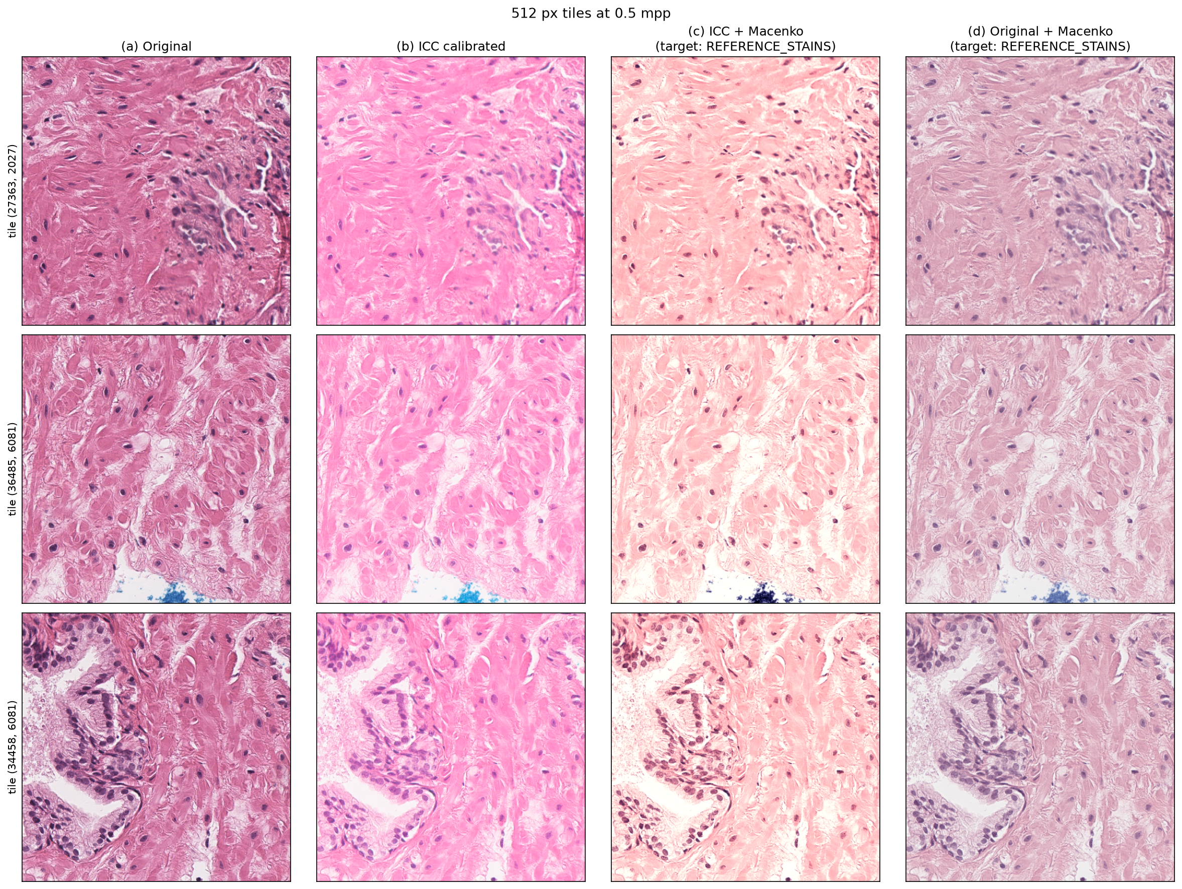Three 512 px tiles at 0.5 µm/px: (a) as stored, (b) after ICC calibration to sRGB, (c) after ICC and Macenko normalisation to REFERENCE_STAINS, (d) after Macenko normalisation alone, with stains estimated on uncalibrated colours.

The classic REFERENCE_STAINS target gives a pale eosin (as in (c)); pass your own reference tile, e.g. stain_target="my_reference.png", to match your data. Regenerate the figure with uv run --with matplotlib python -m patchology.utilities.plot_color slide.svs [reference.png].

To normalise to your own cohort instead, estimate its stains from a set of slides. estimate_stains estimates each slide's stains as tiling does, writes their median to JSON and lists the slides furthest from it (often a wrong stain type or a failed stain):

python -m patchology.utilities.estimate_stains cohort_stains.json slides/ --max-slides 100

ColorConfig(stain_normalization="macenko", stain_target="cohort_stains.json")

Pass H&E slides only (Macenko assumes two stains), and estimate with the same icc setting you tile with (--icc for icc=True).

Visualization

All functions return a PIL.Image (shown inline in Jupyter; .show() or .save() elsewhere). Tissue is drawn in green and artifacts in red. Tiles from a square grid are drawn as blue boxes, and tiles from a hex grid as black hexagons centred on each tile (tile_shape= and tile_color= override this).

from patchology import visualize_result, visualize_slide

result.overlay()  # masks + tiles on the detection thumbnail
result.overlay(tiles=False)  # tissue mask only
result.overlay(tissue=False, artifacts=False)  # tile grid only
result.overlay(slide=slide, max_size=4096)  # sharper, re-read from the slide

# Any slide / mask / coordinates, e.g. reloaded from a saved run:
visualize_slide(
    slide,
    tissue_mask="out/tissue_mask.png",
    coords=coords,
    tile_size=level0_tile_size,
    max_size=2048,
)

draw_mask and draw_tiles are the numpy building blocks, for composing your own figures.

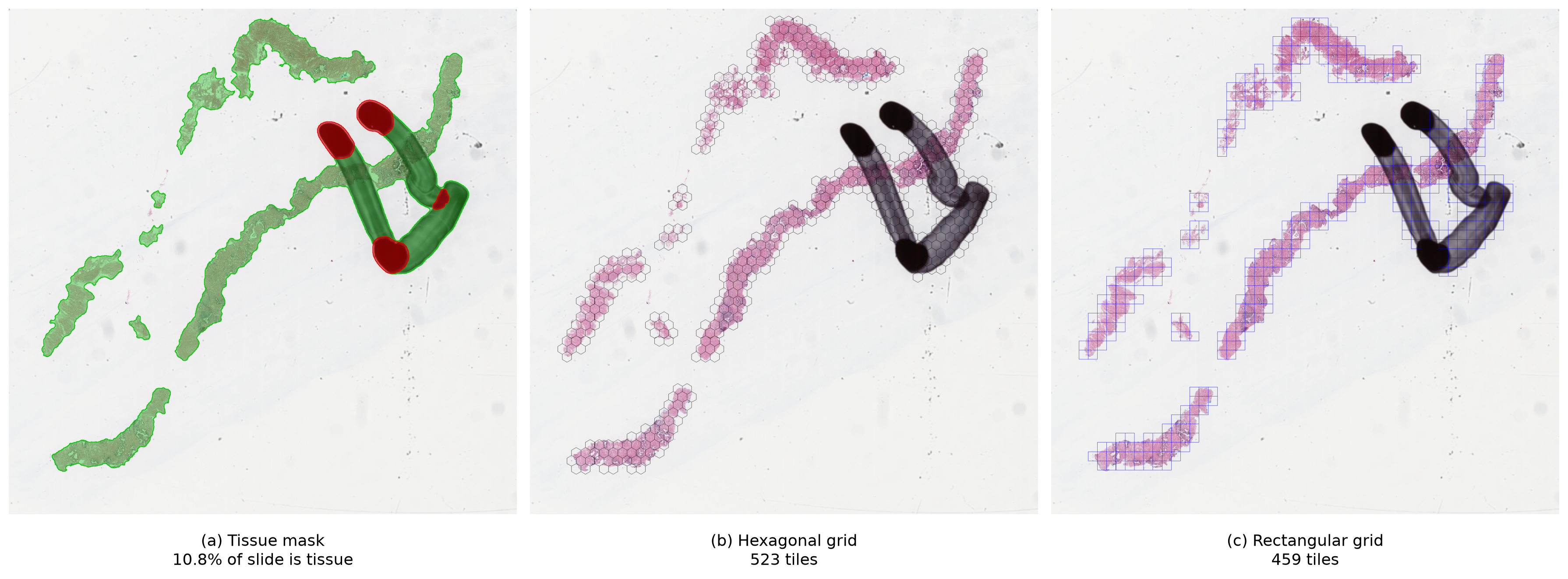512×512 px tiles at 0.5 µm/px, tile_overlap=0, tissue_overlap=0.1.

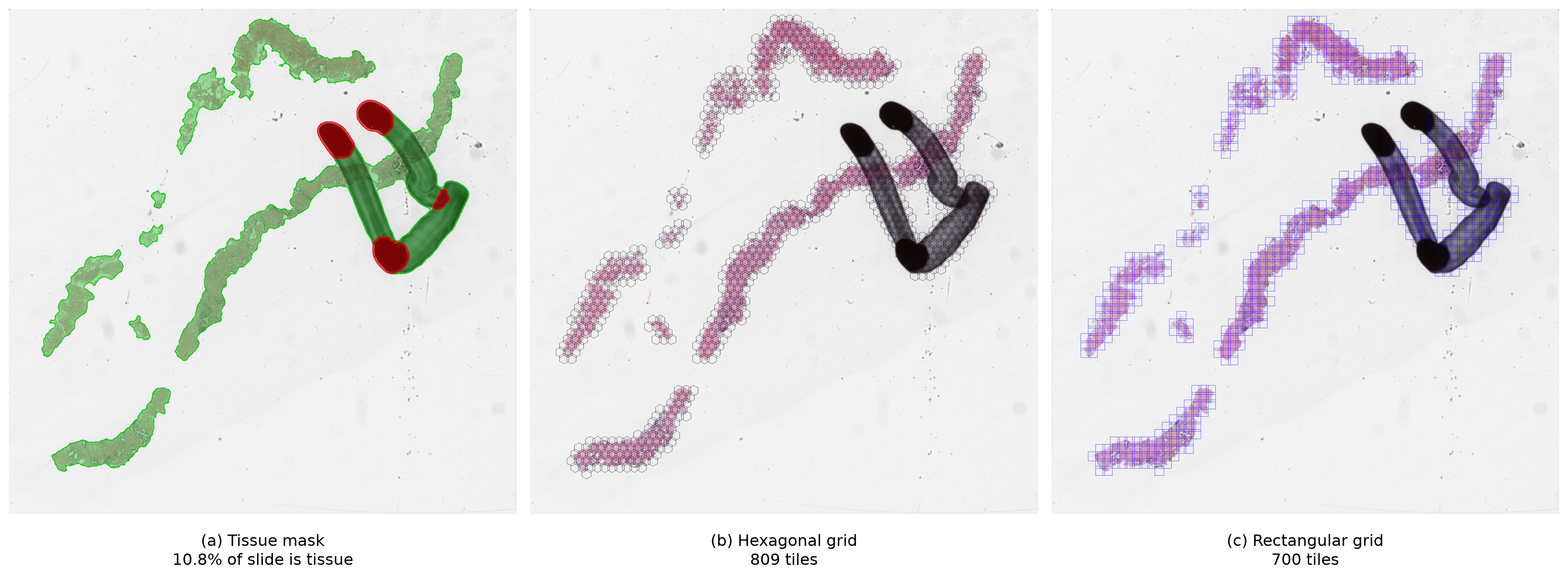Same slide with tile_overlap=0.2.

Logging

Logs (via loguru) show INFO and above by default. Override before running:

export PATCHOLOGY_LOG_LEVEL=DEBUG   # or ALL for everything, WARNING for less

Each library in the family reads its own <PACKAGE>_LOG_LEVEL (e.g. PATHOTRAIN_LOG_LEVEL), so levels are set per library in any import order. If your application configures loguru itself (removes the default handler before importing patchology), that setup is left untouched.

Development

uv sync
uv run pytest
# Backend conformance tests against a real slide:
PATCHOLOGY_TEST_SLIDE=/path/to/slide.svs uv run pytest

Credits

patchology builds on these projects:

• FastSlide: fast whole-slide image reader, one of the two backends.
• OpenSlide: whole-slide image reader, the other backend.
• QuPath: its GeoJSON annotation format is what patchology reads for ROIs and ground truth.

License

Apache License 2.0, see LICENSE. OpenSlide (installed via openslide-bin) is LGPL-2.1 and is used as a separate library; FastSlide is Apache-2.0.